Rare events and quantum correlations

The standard framing of rare event prediction is wrong. People talk about it as a data problem. Not enough crime incidents. Not enough epidemic onsets. Not enough maternal deaths in the training set. The solution, in this framing, is more data. Better surveillance. Longer time horizons. And that framing is wrong in a way that makes the problem harder, not easier.

Frankly, rare events are not rare because they are unpredictable. They are rare because the conditions that produce them are brief. An epidemic doesn’t emerge randomly from a population. It emerges from a specific configuration — mobility patterns, immunity gaps, seasonal humidity, healthcare saturation — that briefly aligns, tips, and then either resolves or cascades. The event itself is short. The preconditions are long and diffuse. And the preconditions are almost always visible in the data if you know where to look.

The actual problem is that classical models look in the wrong places. They look at individual features. Is unemployment high? Is temperature unusual? Is population density above some threshold? These questions make sense if rare events are caused by individual variables crossing thresholds. But they are not. They are caused by variables entering specific relationships with each other. The signal is in the correlation structure, not in the marginals.

I. WHAT CORRELATIONS ACTUALLY MEAN

When epidemiologists talk about risk factors, they mean marginals. Smoking increases lung cancer risk. Poverty increases crime. These are statements about individual variables averaged over populations. They are useful for policy. They are not useful for prediction at the case level.

Prediction requires knowing how features relate to each other in the specific configuration that precedes the event. For instance, the question is not “is unemployment high” but “when unemployment is high and housing density is above median and the last local crime incident was within 60 days — does the crime rate in this part of Oshodi increase faster than the regional trend?” That is a three-way interaction.

Classical logistic regression can’t represent it without explicit feature engineering. Gradient boosted trees will find it only if you have enough rare events to split on all three variables in the right order, which you usually don’t. Pftt

So, the geometry of the problem is roughly this. Our data lives in a high-dimensional space — let’s call it D dimensions for D demographic features per observation. Common events cluster in one region of that space. Rare events cluster in a different region, usually thinner and more elongated, lying along a lower-dimensional manifold that cuts through the common-event region at an angle. The rare-event manifold has structure. It has a specific shape determined by the correlations that produce the event. That shape is what you are trying to learn.

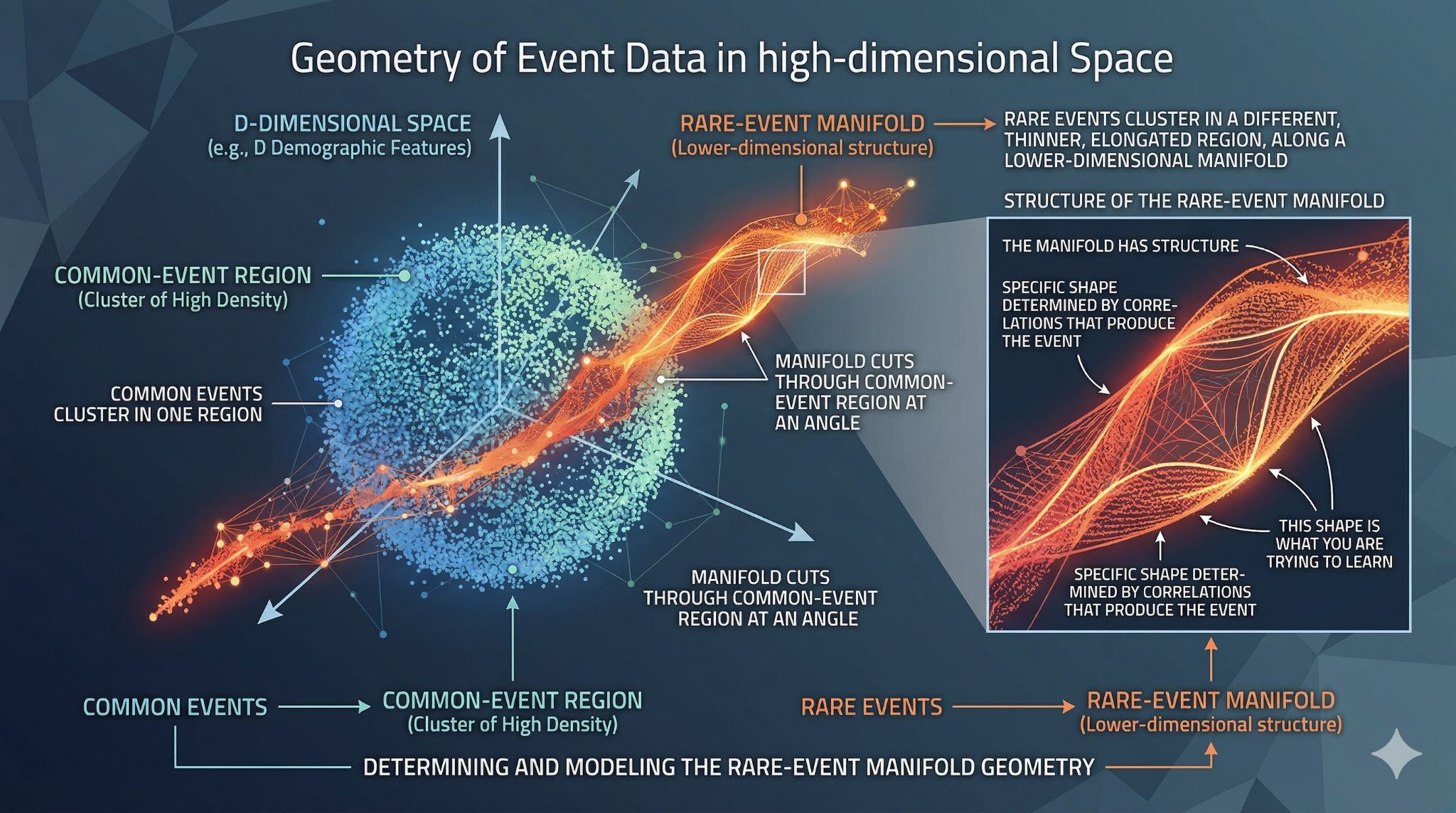
I tried to illustrate the gibberish I just wrote, I hope this image helps you understand better.

The signal is in the correlation structure, not in the marginals. Classical models almost never look there.

Classical models fail at this because they don’t have enough rare events to estimate the geometry of that manifold directly. If we have 10,000 observations and 50 rare events, you have 50 points in a 50-dimensional space. That’s rank-deficient by definition. You cannot estimate a covariance matrix from it. We cannot learn the shape of the manifold. We are always working with a projection of a projection, losing information at every step.

II. WHAT CHANGES IN A QUANTUM ENVIRONMENT

Unlike in classical models, a Quantum Boltzmann Machine does not learn a probability distribution by memorizing examples. It learns a Hamiltonian which is a physical description of the energy landscape of the system. The equilibrium state of that Hamiltonian, which is what you train toward, is a density matrix that encodes the full joint distribution over your features, including all higher-order correlations, without you specifying which correlations to look for.

This matters for rare events in a specific way. The Hamiltonian you learn applies to the whole distribution, common events and rare events together. The rare events are not a separate model. They are a region of the same learned energy landscape, just at higher energy. And because the Hamiltonian is a continuous object, you can sample from that high-energy region directly.

The mechanism is temperature. The equilibrium distribution at inverse temperature β concentrates around low-energy states — common events — at high β, and spreads across the whole energy landscape at low β. By modulating β, you move continuously along a spectrum from the modal distribution to something that upweights rare events without fabricating them. You are not generating synthetic data in the usual sense. You are drawing samples from a different regime of the same learned physical system. The correlation structure — the shape of the manifold — is preserved. What changes is the sampling density.

On a 105-qubit processor, the hidden layer of the QBM operates in a Hilbert space of dimension 2^105. That is more states than atoms in the observable universe. The practical consequence is that the hidden units can represent correlation structure of an order that no classical model can efficiently approximate. Three-way interactions, four-way interactions, interactions that involve features we would never have thought to engineer — they are all captured implicitly in the learned Hamiltonian. Not because the model was told to look for them, but because the quantum structure of the hidden layer can represent them.

III. EXTRACTING WHAT THE MACHINE LEARNED

Training the QBM is not the hard part. The hard part is reading out what it learned in a form that is scientifically interpretable. You want to know: which features are most tightly correlated in the precondition state? Which correlations change as you move toward the rare event? Those questions are what the correlation extraction step answers.

The workflow is roughly as follows. After training, you clamp the visible units corresponding to the outcome — epidemic onset, crime spike, maternal complication — to their rare-event values. The remaining visible units now sample from the conditional distribution: features given that the event is occurring. You take many measurement shots from this conditional state in randomly chosen Pauli bases. From those shots, using classical shadow tomography, you reconstruct the pairwise and higher-order correlators over the feature space.

The number you care about is the connected correlator: the covariance between features i and j in the rare-event conditional distribution, minus the covariance in the unconditional distribution. Where this difference is large, the relationship between those two features changes as you approach the event. That change is your predictive signal. It is not a rule-based flag. It is a description of how the system reconfigures itself before something happens.

For crime prediction in urban demographics, this might show us that the relationship between housing churn rate and lighting infrastructure quality becomes strongly positive in the weeks before a spike — not because either variable alone is predictive, but because rapid population turnover in underlit areas creates a specific vulnerability that neither factor creates alone. You would never have engineered that interaction. The QBM finds it because the quantum correlations in the hidden layer are capable of representing it.

IV. THE HONEST ACCOUNTING

None of this is proven at scale. The theoretical argument for quantum advantage in distribution learning is solid. The empirical benchmarks at 105 qubits on real demographic data do not yet exist. Part of the value of this research program is producing them.

What we know is this. Rare event prediction is a problem where the failure mode of classical methods is structural, not just computational. They fail because they cannot represent the geometry of the rare-event subspace in high-dimensional data. QBMs have a structural property — the quantum correlations in the hidden layer — that could address exactly that failure mode. The question is whether the theoretical advantage survives decoherence, gate errors, and the practical constraints of real hardware.

That question has not been answerable until now. At 50 qubits, decoherence wins. At 105 qubits, with Willow’s two-qubit gate fidelity at 99.7 percent, quantum correlations in the hidden layer survive long enough to do work. This is the first moment in the history of the hardware where testing the theoretical advantage on real data is physically possible.

The applications are not abstract. Epidemic onset prediction in West African populations. Crime spike forecasting in Lagos and Accra. Maternal mortality risk in contexts where clinical records are sparse. These are the exact settings where classical models fail hardest — high dimensionality, rare events, limited labeled data — and where accurate early warning would have the most impact. If the quantum advantage is real, it will show up here first. And if it is not real, finding that out is also worth knowing.

Kossiso Udodi Royce — Electric Sheep Africa, Lagos. Research conducted in partial support of the Google Quantum AI Willow Early Access Program application. Emulation pipeline: sheepq. Edge deployment: Timber Cloud.